!pip install pyro-pplThe following Bayesian LSTM model:
- Learns Temporal Patterns: By using an LSTM layer, it captures the sequential dependencies inherent in financial data.
- Quantifies Uncertainty: The Bayesian treatment of the final layer provides uncertainty estimates, which are critical for risk management.
- Optimizes Performance: Hyperparameter tuning via Optuna ensures the model is well-calibrated.
This following code implements a Bayesian deep learning model for forecasting financial volatility. It retrieves historical S&P 500 data via yfinance, engineers several technical features (like log returns, moving averages, RSI, and volatility), and uses these to build time-series sequences. The central model is a Bayesian LSTM—combining a deterministic LSTM for sequence learning with a Bayesian linear output layer to capture predictive uncertainty. Such a framework is crucial in finance where understanding uncertainty (risk) is as important as forecasting the central tendency.
!pip install optunaData Preparation
- Data Retrieval: Historical S&P 500 price data is obtained via the yfinance API.
- Feature Engineering: Compute log returns, rolling volatility, moving averages (MA₁₀ and MA₅₀), the Relative Strength Index (RSI), and percentage change in volume.
- Normalization & Sequencing: Features are standardized and arranged into sequences (lookback = 21 days) to form the input tensor.
Model Architecture
- LSTM Encoder: The deterministic LSTM layer processes the sequence of features to capture temporal dynamics.
- Bayesian Final Layer: A Bayesian linear layer (with priors on its weights, bias, and noise parameter) produces predictions while modeling uncertainty.
- Inference: Variational inference is performed using Pyro’s SVI with the Trace_ELBO loss, and an AutoNormal guide is used for posterior approximation.
Hyperparameter Tuning
Optuna is used to tune key hyperparameters:
- Hidden Dimension: The number of neurons in the LSTM layer is optimized.
- Learning Rate: The step size for the optimizer is also tuned.
A validation split with early stopping is employed to select the best configuration.
Training & Diagnostics
After tuning, the final model is retrained on the full training set. The training progress is monitored by plotting the ELBO loss over epochs.
Additional diagnostic steps include:
- Volatility Time Series: The historical volatility of the market is plotted.
- Autocorrelation Function (ACF): The ACF plot of volatility confirms temporal dependencies.
- Stationarity Test: An Augmented Dickey-Fuller (ADF) test is conducted.
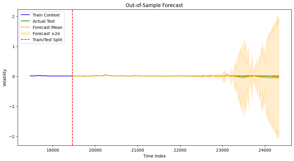
Forecasting
The model performs predictive inference on the test set by:
- Sampling from the posterior to obtain forecast distributions.
- Calculating the mean forecast and uncertainty (±2σ bounds).
The forecasts are visualized alongside the true volatility values, and error metrics (MSE, MAE) are reported.
import torch, numpy as np, pandas as pd, yfinance as yf, matplotlib.pyplot as plt, pyro, warnings, optuna
import torch.nn as nn
from torch.utils.data import DataLoader, TensorDataset
from pyro.nn import PyroModule, PyroSample
import pyro.distributions as dist
from pyro.infer import SVI, Trace_ELBO, Predictive
from pyro.optim import Adam
from pyro.infer.autoguide import AutoNormal
from sklearn.preprocessing import StandardScaler
from statsmodels.graphics.tsaplots import plot_acf
from statsmodels.tsa.stattools import adfuller
from sklearn.metrics import mean_squared_error, mean_absolute_error
warnings.filterwarnings("ignore")
torch.manual_seed(42); pyro.set_rng_seed(42)

# -------------------------
# Data Retrieval & Feature Engineering
# -------------------------
ticker = "^GSPC"
df = yf.Ticker(ticker).history(period="max", auto_adjust=True).reset_index()
if df.empty: raise ValueError("No data retrieved")
df['Log_Return'] = np.log(df['Close']+1e-9).diff()
df['Volatility'] = df['Log_Return'].rolling(21, min_periods=1).std()
df['MA_10'] = df['Close'].rolling(10).mean()
df['MA_50'] = df['Close'].rolling(50).mean()
delta = df['Close'].diff()
gain = delta.clip(lower=0)
loss = -delta.clip(upper=0)
avg_gain = gain.rolling(14, min_periods=1).mean()
avg_loss = loss.rolling(14, min_periods=1).mean()
df['RSI'] = 100 - 100/(1+avg_gain/(avg_loss+1e-8))
df['Volume_Change'] = df['Volume'].replace(0,np.nan).pct_change().fillna(0)
cols = ['Log_Return','Volatility','MA_10','MA_50','RSI','Volume_Change','Open','High','Low']
df = df[cols].dropna().replace([np.inf,-np.inf],np.nan).dropna().reset_index(drop=True)
scaler = StandardScaler()
feat_arr = scaler.fit_transform(df[cols])
target = df['Volatility'].values[1:]
lookback = 21
X_list = [feat_arr[i-lookback:i] for i in range(lookback, len(feat_arr)-1)]
y_list = [target[i] for i in range(lookback, len(feat_arr)-1)]
X = torch.tensor(np.array(X_list),dtype=torch.float32)
y = torch.tensor(np.array(y_list),dtype=torch.float32)
train_size = int(0.8*len(X))
X_train, X_test = X[:train_size], X[train_size:]
y_train, y_test = y[:train_size], y[train_size:]

# -------------------------
# Bayesian LSTM Model Definition
# -------------------------
# Bayesian LSTM: deterministic LSTM + Bayesian final layer
class BayesianLSTM(PyroModule):
    def __init__(self, input_dim, hidden_dim, num_layers=1):
        super().__init__()
        self.lstm = nn.LSTM(input_dim, hidden_dim, num_layers=num_layers, batch_first=True)
        self.fc = PyroModule[nn.Linear](hidden_dim, 1)
        self.fc.weight = PyroSample(dist.Normal(0., 1.).expand([1, hidden_dim]).to_event(2))
        self.fc.bias   = PyroSample(dist.Normal(0., 1.).expand([1]).to_event(1))
        self.sigma     = PyroSample(dist.LogNormal(0., 1.))
    def forward(self, x, y=None):
        lstm_out, (h_n, _) = self.lstm(x)
        h = h_n[-1]  # shape: (batch, hidden_dim)
        weight = self.fc.weight
        bias = self.fc.bias
        if weight.dim() == 3:  # vectorized case: (S, 1, hidden_dim)
            S = weight.size(0)
            h_exp = h.unsqueeze(0).expand(S, -1, -1)  # (S, batch, hidden_dim)
            pred = torch.bmm(h_exp, weight.transpose(1, 2)).squeeze(-1) + bias.unsqueeze(1)  # (S, batch)
        else:
            pred = self.fc(h).squeeze(-1)  # (batch)
        sigma = self.sigma
        if pred.dim() == 2 and sigma.dim() == 1:
            sigma = sigma.unsqueeze(1)
        with pyro.plate("data", x.shape[0]):
            # Always sample "obs", whether or not y is provided.
            if y is not None:
                obs = pyro.sample("obs", dist.Normal(pred, sigma), obs=y)
            else:
                obs = pyro.sample("obs", dist.Normal(pred, sigma))
        return obs

# -------------------------
# Hyperparameter Tuning with Optuna
# -------------------------
def objective(trial):
    pyro.clear_param_store()  # clear previous parameters
    hidden_dim = trial.suggest_int("hidden_dim", 32, 128)
    lr = trial.suggest_loguniform("lr", 1e-3, 1e-1)
    model = BayesianLSTM(input_dim=9, hidden_dim=hidden_dim)
    guide = AutoNormal(model)
    svi = SVI(model, guide, Adam({"lr": lr}), loss=Trace_ELBO())
    # Create inner training/validation split from training data (80/20 split)
    inner_size = int(0.8 * len(X_train))
    X_tr, X_val = X_train[:inner_size], X_train[inner_size:]
    y_tr, y_val = y_train[:inner_size], y_train[inner_size:]
    train_loader = DataLoader(TensorDataset(X_tr, y_tr), batch_size=64, shuffle=True)
    best_val_loss = float("inf")
    patience, no_improve = 10, 0
    num_epochs = 50
    for epoch in range(num_epochs):
        for bx, by in train_loader:
            svi.step(bx, by)
        # Evaluate on validation set
        val_loss = 0.
        val_loader = DataLoader(TensorDataset(X_val, y_val), batch_size=64)
        for bx, by in val_loader:
            val_loss += svi.evaluate_loss(bx, by) * bx.size(0)
        val_loss /= len(X_val)
        if val_loss < best_val_loss:
            best_val_loss = val_loss
            no_improve = 0
        else:
            no_improve += 1
        if no_improve >= patience:
            break
    return best_val_loss

study = optuna.create_study(direction="minimize")
study.optimize(objective, n_trials=30)
best_params = study.best_params
print("Best Hyperparameters:", best_params)
# -------------------------
# Retrain Final Model with Best Hyperparameters
# -------------------------
pyro.clear_param_store()
final_model = BayesianLSTM(input_dim=9, hidden_dim=best_params["hidden_dim"])
final_guide = AutoNormal(final_model)
final_svi = SVI(final_model, final_guide, Adam({"lr": best_params["lr"]}), loss=Trace_ELBO())
final_epochs = 100
train_loader = DataLoader(TensorDataset(X_train, y_train), batch_size=64, shuffle=True)
for epoch in range(final_epochs):
epoch_loss = sum(final_svi.step(bx, by) for bx, by in train_loader)
if (epoch+1)%10==0:
print(f"Final Model Epoch {epoch+1}: Loss {epoch_loss/len(X_train):.4f}")# -------------------------
# Diagnostics & Forecasting
# -------------------------
plt.figure(figsize=(12,6)); plt.plot(df['Volatility']); plt.title('Volatility Time Series'); plt.show()
plt.figure(figsize=(10,4)); plot_acf(df['Volatility'], lags=200); plt.title('ACF of Volatility'); plt.show()
adf = adfuller(df['Volatility'])
print(f"ADF Statistic: {adf[0]:.4f}, p-value: {adf[1]:.4f}")
print("Series is likely stationary" if adf[1]<0.05 else "Series is likely non-stationary")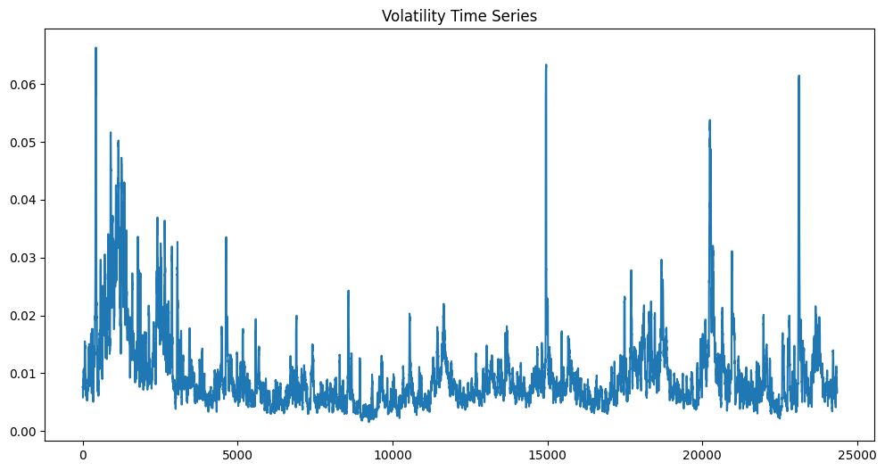
<Figure size 1000x400 with 0 Axes>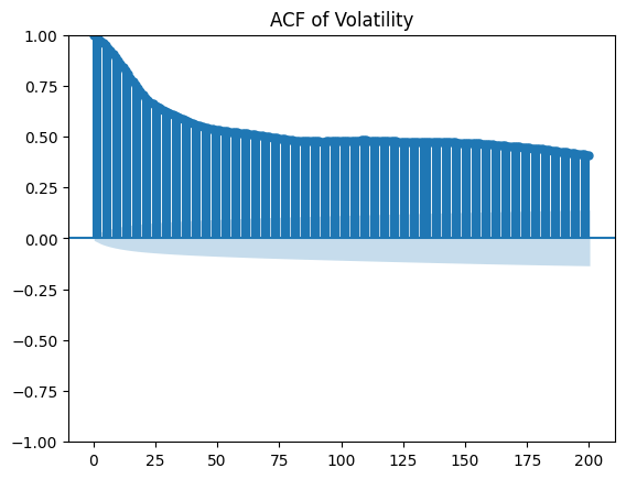
ADF Statistic: -8.9611, p-value: 0.0000
Series is likely stationary
This section performs posterior predictive inference and visualizes the results alongside the true volatility data. final_model & final_guide are the trained Bayesian LSTM model and its corresponding variational guide. They define the learned distribution over the model’s parameters. num_samples=100 tells the Predictive object to draw 100 samples from the posterior. These samples are used to compute the forecast’s mean and uncertainty (standard deviation). return_sites=["obs"] specifies that we want to extract the predictions at the “obs” (observation) site of the model. The model’s uncertainty in forecasting volatility is quantified by averaging across these samples (mean and ±2 standard deviations). If the number of samples is too low, uncertainty estimates might be unreliable.
# Predictive inference
predictive = Predictive(final_model, guide=final_guide, num_samples=100, return_sites=["obs"])
samples = predictive(X_test)["obs"]
y_pred_mean = samples.mean(0).detach().numpy().squeeze()
y_pred_std = samples.std(0).detach().numpy().squeeze()
print(f"Test MSE: {mean_squared_error(y_test.numpy(), y_pred_mean):.4f}")
print(f"Test MAE: {mean_absolute_error(y_test.numpy(), y_pred_mean):.4f}")

num_context = 1000 # the most recent number of training points
ctx_idx = np.arange(train_size-num_context, train_size)
fcast_idx = np.arange(train_size, train_size+len(y_test))
plt.figure(figsize=(12,6))
plt.plot(ctx_idx, y_train[-num_context:].detach().numpy(), label="Train Context", color="blue")
plt.plot(fcast_idx, y_test.numpy(), label="Actual Test", color="green")
plt.plot(fcast_idx, y_pred_mean, label="Forecast Mean", color="orange")
plt.fill_between(fcast_idx, y_pred_mean-2*y_pred_std, y_pred_mean+2*y_pred_std,
                 color="orange", alpha=0.2, label="Forecast ±2σ")
plt.axvline(train_size, color="red", linestyle="--", label="Train/Test Split")
plt.xlabel("Time Index"); plt.ylabel("Volatility"); plt.title("Out-of-Sample Forecast"); plt.legend()
plt.show()
Test MSE: 0.0003
Test MAE: 0.0087